
- 稠密光流(对图像中的每个像素点都计算光流)
0. Image Warping
- 一种图像Transform的算法
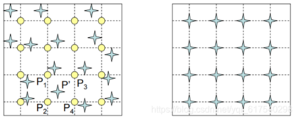
0.1 Forward Warping
1) 概念理解
把source_image中点的值直接warp到destination_image中对应点上
遍历
source image中的每个点p_source,乘以从source image到destination image的affine matrix,将其投影到destination image中得到p_destination,如果p_destination的坐标不是整数,则进行四舍五入取整


这样会产生一个问题:
destination image中有的位置没有从source image中投影过来的点,有的位置有多个从source image中投影过来的点,所以会产生很多空洞,产生类似波纹的效果。

2)代码理解
该部分可以在理解光流之后再回看
- 例子:
0.2 Backward Warping
1)概念理解
把destination_image中的点warp到source_image对应点上,找最近的点的值
遍历destination image中的每个点p_destination,乘以destination image到source image的affine matrix,得这个点在source image中的对应点p_source,令p_destination的像素值等于p_source的值,如果p_source的坐标不是整数,则采用插值逼近的方法进行近似,因此不会产生的Forward Warping的问题。

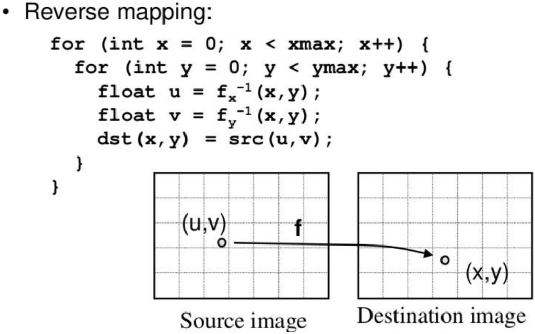
前面是由source_image + f,将source_image每个点映射到dest_image
现在是对dest_image中的每个点,去source_image找答案

2)代码理解
该部分可以在理解光流之后再回看
假设输入图片:
1
2
3
4
1 2 3 4
5 6 7 8
9 10 11 12
13 14 15 16希望将该图片左边两列上移一行,右边两列下移一行。那么x轴不动,在y轴移动
这里移动一个单位对应的值需要注意,正常以为取 (-0.5, 0.5) 就是不动,然后加减1对应移动一个单位。这里是取 (0, 1) 范围时,不动。因此这里以0.5作为中心。对应的光流矩阵:
1
2
3
4
5
6
7
8[[[[0.5,0.5,0.5,0.5],
[0.5,0.5,0.5,0.5],
[0.5,0.5,0.5,0.5],
[0.5,0.5,0.5,0.5]],
[[1.5,1.5,-0.5,-0.5],
[1.5,1.5,-0.5,-0.5],
[1.5,1.5,-0.5,-0.5],
[1.5,1.5,-0.5,-0.5]]]]
1 | import torch |
输出
1
2
3
4tensor([[[[[ 5., 6., 3., 4.],
[ 9., 10., 3., 4.],
[13., 14., 7., 8.],
[13., 14., 11., 12.]]]]], device='cuda:1')仅针对左上角第一个元素(从光流矩阵的角度看),把他替换成左下角第一个元素。这时的理解逻辑是:
对于左上角这个元素,向下位移3个单位找到他的替代点,此时的光流为:1
2
3
4
5
6
7
8reference_flow = torch.tensor([[[[0.5,0.5,0.5,0.5],
[0.5,0.5,0.5,0.5],
[0.5,0.5,0.5,0.5],
[0.5,0.5,0.5,0.5]],
[[3.5,0.5,0.5,0.5],
[0.5,0.5,0.5,0.5],
[0.5,0.5,0.5,0.5],
[0.5,0.5,0.5,0.5]]]]).float().to(device)
3) 图像wrap函数理解
对于上面的
warp_latents_independently函数,通过如下例子进行理解:1
2
3
4
5
6
7
8
9
10
11
12
13
14
15
16
17
18
19
20
21
22
23
24
25
26
27
28
29
30
31
32
33
34
35
36
37
38
39
40
41
42
43
44
45
46
47
48
49
50
51
52
53
54
55
56
57
58
59
60
61
62
63
64
65
66def warp_latents_independently( latents, reference_flow ):
# latents=[[[[ #1,1,1,2,2
# [1,2],
# [3,4]
# ]]]]
# reference_flow = [[[[1,2,3,4], #1,2,4,4
# [2,3,4,5],
# [3,4,5,6],
# [4,5,6,7]],
# [[10,11,12,13],
# [2 ,2 ,2 ,2 ],
# [1 ,3 ,5 ,8 ],
# [1 ,1 ,2 ,2 ]]]]
device = latents.device
_, _, H, W = reference_flow.size() #1,2,4,4
b, _, f, h, w = latents.size() #1,1,1,2,2
assert b == 1
coords0 = coords_grid(f, H, W, device=latents.device).to(latents.dtype)
#coords0 = [[[[0,1,2,3], #1,2,4,4
# [0,1,2,3],
# [0,1,2,3],
# [0,1,2,3]],
# [[0,0,0,0],
# [1,1,1,1],
# [2,2,2,2],
# [3,3,3,3]]]]
coords_t0 = coords0 + reference_flow
#coords_t0 = [[[[1,3,5,7], #1,2,4,4
# [2,4,6,8],
# [3,5,7,9],
# [4,6,8,10]],
# [[10,11,12,13],
# [3 ,3 ,3 ,3 ],
# [3 ,5 ,7 ,10],
# [4 ,4 ,5 ,5]]]]
coords_t0[:, 0] /= W
coords_t0[:, 1] /= H
coords_t0 = coords_t0 * 2.0 - 1.0
#coords_t0 = [[[[-0.5, 0.5, 1.5, 2.5], #1,2,4,4
# [ 0 , 1 , 2 , 3 ],
# [ 0.5, 1.5, 2.5, 3.5],
# [ 1 , 2 , 3 , 4 ]],
# [[4 , 4.5, 5 , 5.5],
# [0.5, 0.5, 0.5, 0.5],
# [0.5, 1.5, 2.5, 4 ],
# [1 , 1 , 1.5, 1.5]]]]
coords_t0 = T.Resize((h, w))(coords_t0)
#相邻四个取平均:左上角四个:-0.5, 0.5, 0, 1取平均=0.25
#coords_t0 = [[[[0.25, 2.25], #1,2,2,2
# [1.25, 3.25]],
# [[2.375, 2.875],
# [1 , 2.375]]]]
coords_t0 = rearrange(coords_t0, 'f c h w -> f h w c')
latents_0 = rearrange(latents[0], 'c f h w -> f c h w')
warped = grid_sample(latents_0, coords_t0,
mode='nearest', padding_mode='reflection')
# warped=[[[[ #1,1,1,2,2
# [2,1],
# [4,1]
# ]]]]
warped = rearrange(warped, '(b f) c h w -> b c f h w', f=f)
return warpedgrid_sample函数理解:
输入参数:
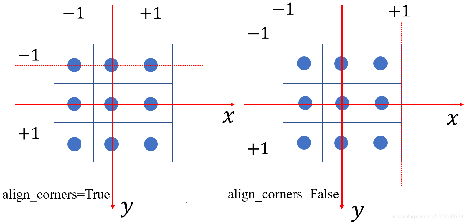
inputgridmode:采样的方式,nearest就是最邻近采样,bilinear是双线性插值。padding_mode:边缘的处理模式,zeros是边缘补充部分为0,border是边缘补充部分直接复制边缘区域,reflection是边缘补充部分为根据边缘的镜像align_corners:当align_corners=True时,坐标归一化范围是图像四个角点的中心;当align_corners=False时,坐标归一化范围是图像四个角点靠外的角点。如下,其中每一个方格代表一个像素,并且像素坐标在方格中央
举例:
1  2  3  4
5  6  7  8
9  10 11 12
13 14 15 16
17
18
19
20
21
22
23
24
25
26
27#输入图片
test = tensor([[[[1., 2., 3.],
[4., 5., 6.],
[7., 8., 9.]]]])
#采样点
sample_one = torch.zeros(1,1,1,2)
sample_one [0][0][0][0] = -1 # x
sample_one [0][0][0][1] = -1 # y
sample_two = torch.zeros(1,1,1,2)
sample_two [0][0][0][0] = -2/3 # x
sample_two [0][0][0][1] = -2/3 # y
sample_thr = torch.zeros(1,1,1,2)
sample_thr [0][0][0][0] = -0.5 # x
sample_thr [0][0][0][1] = -0.5 # y
#采样
result_one = torch.nn.functional.grid_sample(test,sample,mode='bilinear',padding_mode="zeros",align_corners=True) #左图,(-1, -1)
print(result_one )
result_two= torch.nn.functional.grid_sample(test,sample_two ,mode='bilinear',padding_mode="zeros",align_corners=False)
print(result_two) #右图,(-2/3, -2/3)
result_thr= torch.nn.functional.grid_sample(test,sample_thr ,mode='bilinear',padding_mode="zeros",align_corners=True)
print(result_thr) #左图,双线性插值(1*0.5+2*0.5)*0.5+(4*0.5+5*0.5)*0.5=3
计算方式:继续上一节的例子
1
2
3
4
5
6
7
8
9
10
11# latents=[[[[ #1,1,1,2,2
# [1,2],
# [3,4]
# ]]]]
#coords_t0 = [[[[0.25, 2.25], #1,2,2,2输入grid_sample时还要做reshape
# [1.25, 3.25]],
# [[2.375, 2.875],
# [1 , 2.375]]]]根据输入的参数 reflection ,使用反射填充进行归一化
- 第一个坐标点:
(0.25, 2.375)- x=0.25 在范围内,无需处理。
- y=2.375 → 反射为
1 - (2.375 - 1) = -0.375。 - 处理后坐标:
(0.25, -0.375)。
- 第二个坐标点:
(2.25, 2.875)- x=2.25 → 反射为
1 - (2.25 - 1) = -0.25。 - y=2.875 → 反射为
1 - (2.875 - 1) = -0.875。 - 处理后坐标:
(-0.25, -0.875)。
- x=2.25 → 反射为
- 第三个坐标点:
(1.25, 1.0)- x=1.25 → 反射为
1 - (1.25 - 1) = 0.75。 - y=1.0 在边界上,无需处理。
- 处理后坐标:
(0.75, 1.0)。
- x=1.25 → 反射为
- 第四个坐标点:
(3.25, 2.375)- x=3.25 → 多次反射后为
-0.75。 - y=2.375 → 反射为
1 - (2.375 - 1) = -0.375。 - 处理后坐标:
(-0.75, -0.375)。
- x=3.25 → 多次反射后为
- 第一个坐标点:
根据参数nearest,归一化坐标转像素坐标
转换公式:
pixel = (normalized + 1) * (size / 2) - 0.5(align_corners=False)。- 第一个坐标点:
(0.25, -0.375)- x:
(0.25 + 1) * 1 - 0.5 = 0.75→ 四舍五入到 1。 - y:
(-0.375 + 1) * 1 - 0.5 = 0.125→ 四舍五入到 0。 - 值:
input[0, 0, 0, 1] = 2。
- x:
- 第二个坐标点:
(-0.25, -0.875)- x:
(-0.25 + 1) * 1 - 0.5 = 0.25→ 四舍五入到 0。 - y:
(-0.875 + 1) * 1 - 0.5 = -0.375→ 反射后为 0.375,四舍五入到 0。 - 值:
input[0, 0, 0, 0] = 1。
- x:
- 第三个坐标点:
(0.75, 1.0)- x:
(0.75 + 1) * 1 - 0.5 = 1.25→ 反射后为 0.75,四舍五入到 1。 - y:
(1.0 + 1) * 1 - 0.5 = 1.5→ 反射后为 0.5,四舍五入到 1。 - 值:
input[0, 0, 1, 1] = 4。
- x:
- 第四个坐标点:
(-0.75, -0.375)- x:
(-0.75 + 1) * 1 - 0.5 = -0.25→ 反射后为 0.25,四舍五入到 0。 - y:
(-0.375 + 1) * 1 - 0.5 = 0.125→ 四舍五入到 0。 - 值:
input[0, 0, 0, 0] = 1。
- x:
- 第一个坐标点:
最终输出:
1
2[[[[2, 1],
[4, 1]]]]
1. 光流(optical flow)
光流是一个二维速度场,表示
每个像素pixel从参考图像到目标图像的运动偏移。 数学定义如下:- 给定两个图像img1,img2 $\in R^ {HW3}$
- flow $\in R^ {HW2}$ ,其中channel=2分别描述水平和垂直方向的像素位移。
这里还要注意的一点:像素坐标偏移量的
大小**当然就是通过**光流数组中的数值大小**体现出来的,而偏移的**方向是通过光流数组中的正负体现出来的。在x方向上,正值表示物体向左移动,而负值表示物体向右移动;在y方向上,正值表示物体向上移动,而负值表示物体向下移动。